Just how good are marine nature-based solutions?

The recent report from the British Ecological Society has reviewed a wide range of Nature-based solutions for climate change mitigation. It does clearly state, in multiple locations, that while there are many benefits of NbS, they are not a substitute for heavy emissions cuts. Lots of different habitats and landscapes can capture CO2, but just how much?

This article is a very rough set of calculations based on the figures in the marine chapter of the report. It shouldn’t be treated as fully scientifically sound (unlike the figures from the report itself), nor used to measure any kind of net zero target.

Disclaimer aside (but please bear it in mind) – how good are the oceans at offsetting emissions?

The answer – currently, even restoring seagrass and saltmarsh habitats, less than 100th of the UK emissions. However, before getting too despondent, NbS are NOT a substitute for emission reduction. If we can move to a per-capita footprint, roughly the size of Kenya, then we get to about 15% of emissions absorbed.

Of course, the UK is small, even in terms of its EEZ (outside of overseas territory) and densely populated. Scaling up the figures (with lower certainty) to the entire world, and assuming we can all reduce per-capita footprints to that of an average Kenyan, just over 50% of emissions can be sequestered by the ocean. This may be an underestimate too – with healthier oceans, come better fish stocks, greater productivity, and algae and phytoplankton increases will all boost these figures.

So, marine NbS can play a huge role in addressing climate change, and address biodiversity issues too. However, this only applies if we can make big emissions cuts in the very near future.

Calculations

Quick calculations – carbon sequestration in the UK and globally

This post is designed to create a few simple ‘back of an envelope’ calculations to estimate the benefits of marine NbS in the UK. The figures are taken from the marine and coastal chapter of the British Ecological Society’s Nature-based Solutions report. 

92% of seagrass has potentially been lost. Currently around 8,400 ha of seagrass exists in the UK. 

8400/0.08 (the 8% remaining) = 105000 ha of seagrass

New seagrass captures around sequesters CO2 at the rate of 1.3 tonnes per hectare per year, moving to around 5 tonnes for fully established seagrass beds

= 136000 tonnes per year if newly restored

> 500,000 tonnes once better established

Saltmarsh through shoreline management plans in the UK

Around 3000 ha new saltmarsh by 2030

Restored saltmarsh sequesters CO2 at 3.8 tonnes CO2 per hectare per year

So, 11,400 tonnes CO2 per year from new saltmarsh

  • 46,000 ha of existing saltmarsh sequestering at around 5 tonnes per year

=11,400 + (46,000*5) = 241,400 tonnes CO2 per year

Coastal shelf sediments 388,000 tonnes per year. Coastal shelf is 9% of UK waters. However, most benthic habitats are sand/mud.

So – (388,000 / 0.09) / 2 (as ‘safety factor’ other sediments may be worse) = 2,155,556 tonnes per year.

Boosting phytoplankton and seaweed growth could boost this even further.

So, UK seas, excluding overseas territory ~ 2,750,000 tonnes CO2 per year.

Currently UK produces over 350 million tonnes CO2 per year, or 5.8 tonnes per person. However, Kenya’s per capita emissions are around 0.3 tonnes per person, meaning UK could produce 18.2 million tonnes (or less) with big emissions cuts. 

UK is highly populated and relatively small. UK waters are 773,676 km2 (excluding overseas territories)
Globally the seas cover 361 million km2 or 466 times more. As a very rough calculation as lots changes with location, and the UK also has more coastal habitat than ‘average’ ocean, the sea may be able to sequest in the range of 1,281,500,000 tonnes of CO2 per year. With a population of 8 billion people, and emissions per capita equivalent to Kenya at present, that’s a total emissions scenario of 2.4 billion tonnes CO2 per year. Roughly half of this, with considerable potential for higher figures, could be sequestered by the oceans, if they are restored and protected to optimal condition.

Posted in Uncategorized | Comments Off on Just how good are marine nature-based solutions?

UK’s calls to protect 30% of seas

Yesterday, the DEFRA, the environmental section of the UK government, has supported international calls to designate and protect 30% of the world’s oceans as marine protected areas (MPAs).

My twitter feed has gone a bit mad since with so many comments on this announcement being made, so hopefully this will help clarify my position, and establish some facts around the recent interest in MPAs.
Firstly, more protection is great. The announcement is welcome. It’s policy which has been informed by scientific research. So why are so many people, myself included, sceptical about this?

To most people, it would seem obvious that you can’t fish in a marine protected area, so therefore they help preserve fish stocks. There’s only one problem with this statement, and that is that it isn’t true. There’s no legal definition of what an MPA is and fishing is allowed in most MPAs. In fact, some MPAs allow almost any activity to occur in them, and some even seem to have less strict requirements around fishing than exist outside of the MPAs.

The Convention for Biological Diversity (CBD) set international targets for MPAs of 10% of the surface of the ocean. While these targets have not been met, there has been considerable progress in the last few years. However, how effective the MPAs really are is a matter of debate.
The UK has 36% of its seas designated as MPAs most of which have been designated in the last 10 years. In England (but not Wales or Scotland) these are mainly in the form of Marine Conservation Zones (MCZs). MCZs are legally defined, and certain ‘features’ which are either specific habitat types or specific species are protected in these areas. However, the vast majority have no management measures in place, and no restrictions on activities which can take place within them. They are frequently accused of being ‘paper parks’ with no real measures in place for protection.

The UK has also designated large MPAs in its territorial waters. Chagos in the Indian Ocean is the best example, covering a quarter of a million square miles of ocean. The Chagos MPA is a no-take marine reserves, meaning that fishing isn’t allowed in the area at all. Chagos has found to be an effective MPA, enhancing stocks of overfished species such as bigeye tuna. Other big, offshore MPAs have been established in many territorial waters around the world, however, in some cases, these look like they have been designed to meet the MPA area targets assigned by the CBD – for example, the Easter Island MPA had very little fishing activity in the area before the designation.

It is important to realise that MPAs don’t have to be no take marine reserves to be effective. MPAs can serve different purposes – for example, protecting a fragile habitat such as coral reefs or seagrass from destructive fishing methods – but still allowing some small-scale fishing using non-destructive techniques can do two things. Firstly, it can protect important marine habitats, and secondly, it may allow local support for the MPA in the first place, where as an MPA banning fishing altogether may face opposition from the local community. The large Chagos MPA was only established as the islands are unpopulated (or more accurately, the population has previously been removed). Creating some no take areas, but ‘zoning’ MPAs to allow some fishing in other areas can also be effective. In fact, a recent study has shown that no-take zones close to areas of high human activity can show the highest benefits in terms of increased fish biomass. The same study shows that isolated no-take MPAs show the biggest effect in increasing large predator biomass (i.e. are more effective in protecting big fish such as sharks). In short, a diverse range of MPAs need to be created, but they do need to be monitored and have some kind of restrictions on activity, and create changes to fishing practices occurring in the area to be effective.

The UK’s approach to MPAs has been derided by the Environmental Audit Committee. So, while the announcement of support for 30% of oceans to be protected is welcome, it is necessary to ensure what we have already got is fit for purpose.

Posted in Uncategorized | Comments Off on UK’s calls to protect 30% of seas

Free NERC funded course – Management of Marine Protected Areas using Bayesian Belief Networks

1st December 2017 to 23rd March 2018 – Online

This course focusses on integrating diverse data for effective environmental management – with examples focussing on Marine Protected Areas – but also suitable for any kind of environmental management problems. No knowledge of statistics (Bayesian or otherwise) is required – this is not an in-depth statistical course, but a guide to synthesising data and making robust decisions based on data and using simple and intuitive models embedded in Microsoft Excel worksheets.

Successful marine protected areas (MPAs) need to fulfil a wide range of functions, from protecting ecological indicators such as fish stocks or biodiversity through to maintaining stakeholder engagement and ensuring sufficient economic benefit can be obtained from the MPA and surrounding area. These functions are multidisciplinary, and in many cases, can be antagonistic in nature.

Data to support scientific and management decisions comes in a wide variety of formats, from conclusive outcomes of rigorous meta-analysis at one end of the scale, to anecdotal stories from local fishers at the other. Integrating multiple data sources to provide interdisciplinary information in a manner transparent manner to stakeholders may therefore seem an impossible challenge, yet through this online course you will be guided through how this can be done in a simple and easy to understand manner.

The training programme is run online by Bournemouth University with contributions from JNCC, the Marine Management Authority and Natural England. Places for 25 students will be offered FREE OF CHARGE due to funding of the course by NERC. This will include access to the full set of resources, and comprehensive online support and help throughout. Places will be prioritised for NERC funded PhD students (including those recently completed), however, other applications will be considered form other applicants, including those with other PhD funding or working professionally. The course is accredited for delivery at postgraduate level, and successful completion will result in 20 level 7 credits.

For further information, or to apply, please contact the course leader – Dr Rick Stafford at rstafford@bournemouth.ac.uk. To apply, please include the following information:

Current status (e.g. PhD student, recently completed PhD, Post-doc, Work in industry)
Current funder for work (e.g. NERC, ESRC, University funded, or other)
When did you complete your PhD (if relevant)
Country of residence (e.g. UK)
A brief (max 100 words) description of your academic or professional interest in the course

Posted in Uncategorized | Comments Off on Free NERC funded course – Management of Marine Protected Areas using Bayesian Belief Networks

On open letter to Kelly Slater’s call for a Reunion shark cull

Kelly Slater is a surfing legend, he’s also a keen supporter of environmental issues, which is why his recent comments about a shark cull for Reunion Island are so off the mark. However, he has called for evidence to counter his claim. As a surfer, marine biologist and shark enthusiast in general, this seems like a good reason put together a scientifically defensible reason as to why shark culls won’t work, and maybe even make the problem worse.

Before starting, I would like to clarify that Kelly’s calls for evidence to counteract calls for culling are a responsible thing to do (although arguably, calling for a cull before researching this may not be). He has received a huge amount of abuse on social media, and very little in the way of constructive arguments against culling. I do think the calls for a cull were a genuine response of concern for victims of the attacks. However, I hope to address here that 1) there is no evidence that shark attacks are out of control in Reunion and they pose a low risk, 2) there is a likely reason for a ‘slight’ increase in the number of attacks over time, 3) culling may make the problem of attacks worse. The links all point to peer reviewed journal articles – while these are official links, you may find you can obtain access to them without paying by copying and pasting the article title into Google or Google Scholar.

The Reunion problem in numbers

The headlines are 20 shark attacks since 2011 (eight of which have been fatal). However, 2011 itself saw five attacks, meaning there have been less than three per year on average since 2012. Scientific studies have shown that the rate is slowly increasing (see below for why), and on long-term data collected since 1980, typically there would now be about two attacks per year. So, with the exception of 2011, nothing major has changed, there hasn’t been a recent surge of attacks that can be statistically validated as different from long-term trends.

The risk is also relatively low. The population of Reunion is around 850,000 with another 405,000 visitors each year. As a quick sweeping assumption, if half of these people go in the sea, then that means going in the sea in a typical recent year means an approximately 1 in 200,000 chance of being attacked by a shark. The odds of dying in a transportation accident in 2013 were approximately 1 in 48,000, over four times higher than even being bitten by a shark in Reunion.

Reasons for increasing attacks

Since 1980, there has been a steady but small increase in the risk of a shark attack on Reunion Island. To some extent, this can be attributed to more tourism and more water related activities. Simply put, if sharks bite humans randomly (albeit with a very low probability of doing so), then more humans in the water will mean more bites. However, there are also other issues effecting likely shark bite rates in Reunion. While many theories exist, including over fishing of prey species, a recent study suggests that for Reunion, the main issue is a rise in poorly regulated agriculture. The study states: “Agriculture […] represents an important component of the island’s economy. However, run-off and waste-water are poorly contained.” Agricultural run-off affects water clarity, and therefore sharks’ vision. It is well known that areas of poor visibility are the site of higher numbers of shark attacks. Indeed, the attack on a bodyboarder last week was in a river mouth (which had been closed to all water users by the authorities, due to increased risk of shark attacks).

The problems with culling

Bull sharks (the most likely species thought to have caused the majority of attacks) are seasonal visitors to Reunion. While studies have shown good site fidelity for bull sharks (many return to the same site each year), some do not, and other new individuals arrive. Culling may reduce the population in one season, or even for a few seasons, but it will have little mid- to long-term effect on numbers and can not eliminate the risk of an attack.

Attracting sharks (to catch them or cage dive) usually involves the use of chum (dead fish, blood and oil thrown into the water). Ultimately the use of chum may lead to further attacks on humans, and could attract them into shallower water. The evidence is far from certain, but a recent review of scientific literature says: “We are not aware of any published studies that have examined [whether chumming increasing shark attacks] and therefore, this is certainly an area requiring further research. However, research on a variety of other species has shown that some increased risk of aggression toward humans is possible in provisioned animals.”

Conclusions

Sharks are apex predators which control marine ecosystems and have even been shown to help alleviate climate change by storing or regulating carbon dioxide release. The risk of a shark attack at Reunion is very low, and culling is unlikely to be effective and may even be counterproductive. The solution to preventing attacks is to respect sharks, learn about their behaviour, and avoid more dangerous areas. Along with that, we need to protect the ocean from over fishing (so sharks have food) and pollution (so they can identify humans from their main prey)– as protecting the ocean also protects us from the risk of attack.

Posted in Uncategorized | Comments Off on On open letter to Kelly Slater’s call for a Reunion shark cull

Save the sharks, they prevent climate change!

We already know and can read about the effects of unsustainable fishing. Reduced catches of cod and more costly fish and chips are just part of the message, which can go as far as to include the ‘jellyfish soup’ predictions of Richardson et al. (2009). Collapse of some important predatory fish stocks could (and has) resulted in increases in jellyfish in the ocean, with a further consequence of this being it is also more difficult for fish stocks to recover once jellyfish have established themselves.

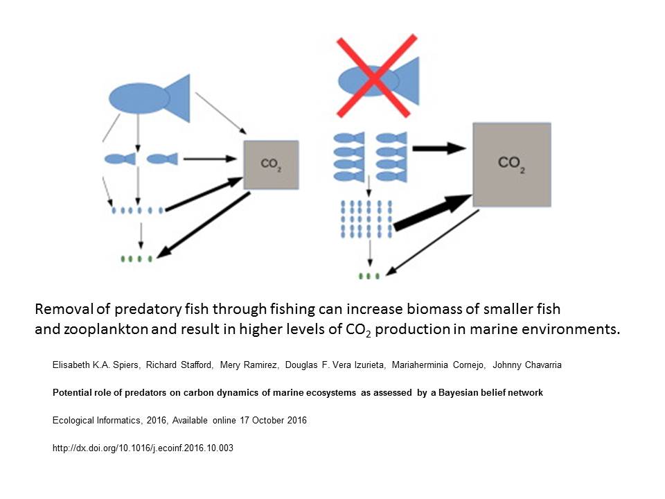
However, our recent paper (Spiers et al., 2016), demonstrates the potential role of predatory fish, including sharks, and other large marine predators such as whales and dolphins, of influencing the carbon budget of the ocean. In short, reducing the numbers of predators may increase carbon dioxide production of the ocean’s ecosystems and result in greater levels of climate change.

s1574954116301820-fx1

The reason is simple, and something almost every student of biology from GCSE or high school upwards will have been taught – trophic inefficiency. Energy (and biomass) is lost as it passes up the food chain. Typically only 10% is passed from predators to prey. So, removing large numbers of predators (and almost all commercial fish we eat are predatory and a long way up the food chain), results in greater levels of biomass further down the foodchain. In the marine environment, this is normally zooplankton and smaller fish. Studies have shown that respiration is proportional to biomass, so a greater biomass of animals means more carbon dioxide production.

While our study is based on a theoretical model, studies on the role of predators on carbon production have been conducted before, in simple systems consisting of only a few species (Atwood et al., 2013; Strickland et al., 2013). Again, they have shown that carbon production can be increased by removing the top predators from the system. More recent work has also demonstrated how predators can effect feeding of prey species and subsequent storage of carbon in marine ecosystems (Atwood et al., 2015). Furthermore, there are other studies such as that by Nicol et al. (2010) that demonstrate the potential role of whales on climate change, though providing nutrients for phytoplankton (the ‘plants’ of the sea) to grow (largely by transporting iron across thermoclines, by feeding at depth and defecating at the surface, allowing these nutrients to come to the surface waters where light is also available for photosynthesis).

It is important to realise the negative effects that abusing ocean ecosystems are having, and to begin to realise the potential consequences are far more far reaching than just for the fish being removed. Despite the recent reduction in demand for shark fin soup, shark finning is still continuing at a very high level in many areas of the world, decimating shark populations even from the levels present 20 years ago. Even sustainable fishing practices involve reduction of fish stocks (typically to half of their natural size), as this allows the greatest catch to be taken each year – and as such, even sustainable fishing could have big effects on ocean carbon production.

However, there are positives from this research too. Allowing predatory fish, sharks, whales and other marine animals to increase (i.e. their populations to recover), will mean that carbon production of the ocean is likely to decrease (from current levels). Creating sustainable fisheries (as a first step), keeping the ban on commercial whaling and outlawing (and enforcing existing bans) on shark finning will have a double positive effect. Not only will numbers of these large, beautiful and enigmatic creatures increase, but also the amount of carbon dioxide entering the oceans (causing acidification) and the atmosphere (causing climate change) will be reduced.

Read the full paper here: http://dx.doi.org/10.1016/j.ecoinf.2016.10.003

Contact me for more information at rstafford – at – bournemouth – dot – ac – dot – uk

References:

Atwood, T.B., Hammill, E.,,Greig, H.S., Kratina P., Shurin J.B., Srivastava D.S., Richardson J.S. (2013) Predator-induced reduction of freshwater carbon dioxide emissions. Nature Geoscience, 6, 191-194.

Atwood, T. B., Connolly, R. M., Ritchie, E. G., Lovelock, C. E., Heithaus, M. R., Hays, G. C., et al. (2015). Predators help protect carbon stocks in blue carbon ecosystems. Nature Climate Change, 5,1038-1045.

Nicol, S., Bowie, A., Jarman, S., Lannuzel, D., Meiners, K. M. and Van Der Merwe, P. (2010), Southern Ocean iron fertilization by baleen whales and Antarctic krill. Fish and Fisheries, 11: 203–209.

Richardson, A. J., Bakun, A., Hays, G. C., & Gibbons, M. J. (2009). The jellyfish joyride: causes, consequences and management responses to a more gelatinous future. Trends in Ecology & Evolution, 24, 312-322.

Spiers, E.K.A., Stafford R., Ramirez M., Vera Izurietab D.F., Chavarria J. 2016. Potential role of predators on carbon dynamics of marine ecosystems as assessed by a Bayesian belief network. Ecological Informatics. In press: doi: 10.1016/j.ecoinf.2016.10.003

Strickland M.S., Hawlena D., Reese A., Bradford M.A., Schmitz O.J. (2013) Trophic cascade alters ecosystem carbon exchange. Proceedings of the National Academy of Sciences, 110, 11035-11038.

Posted in Uncategorized | Comments Off on Save the sharks, they prevent climate change!

Champions’ League

I’d like to say that I’ve delayed this post to allow for an update on the predictions of the model – but it really isn’t true, I just haven’t got around to doing it until now. However, all these predictions are made on data available to me at the start of January. Also, since I have very little knowledge of football (since I left Newcastle in 2006), I haven’t been following anything that has happened, and therefore I have an unbiased methodology (a horrible word, possibly actually used correctly here..)

So, the purpose of this work is to predict which teams will finish in the Champions’ league from the UK premiership (the top 4). I’ve already done some work, based on current points and form (see here), which is my hard quantitative data. However, things can change – there is a transfer window in January to buy new players etc. So, expert opinion might be useful too. And, in football, everyone is an expert… So ‘public opinion’ might be useful too.

The data I have are:

The previous points and form data (see here).

‘Expert’ opinion. This was actually difficult to find (as would probably always be the case), so the best I have is a summary of what players each team needs to buy in the transfer window to maximise their success (courtesy of Match magazine – 30th Dec 2014).

Given that transfers could greatly affect the team, I have then created a ‘money’ variable, which basically looks at the likelihood of being able to purchase the recommended players.

Finally, I’ve found a public survey, asking which teams will be the top 4 finishers (from quibblo.com on the 4th Jan 2015).

Of course, these data are in a wide range of forms – so how do I integrate them?

I’m going to convert each data type into a probability (between 0 and 1) of finishing in the top 4. The previous form data are already in this format.

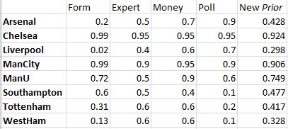
Expert opinion. I’ve used part formula, part intuition to create this. For example, for both Man City and Chelsea, there were no specific signings recommended – however, the tone of writing (as judged by me – so, yes, slightly subjective) was more positive for Chelsea – Man City’s entry said: “..a big name transfer would be a massive boost for the players and fans”, compared to Chelsea: “we’d sign a massive star to make their squad even more unstoppable”. Both are clearly high, as no weaknesses were identified – so Chelsea get a value of 0.95, Man City = 0.9. Other than that, it was relatively simple – one player identified as vital (in a role, such as defence, striker) = 0.6, two players = 0.5, three players = 0.4.

Money. This was very subjective, and wasn’t really researched here. However, it is well known (even by me) that some teams have more money than others. Hence, this looked at the likelihood of being able to buy the players identified above – lower scores for poorer clubs and those needing more players.

Public opinion – This was largely numeric data anyway. Votes were available for each team, in this case, the highest number of votes (26) was for Chelsea – converting to 0.95 probability. Man City and Arsenal were on 22 and 23 votes resperctively  -both getting probabilities of 0.9. Liverpool had 17 votes (p=0.7), Man U 14 (p=0.6), Tottenham had 5 votes (p=0.2), Southampton has 2 votes (p=0.1) and West Ham were not on the list (p=0.1 – all other teams were low, so it is likely if they were included, they would be low too). Obviously there may be bias in here – with people voting for teams they support over true opinion, but largely this is the nature of public opinion, it is bias – and it doesn’t need to necessarily be treated as equal to other data (see below).

The probabilities for each team (as well as the overall probability – prior to interactions) are shown below:

inputData

Integrating the data:

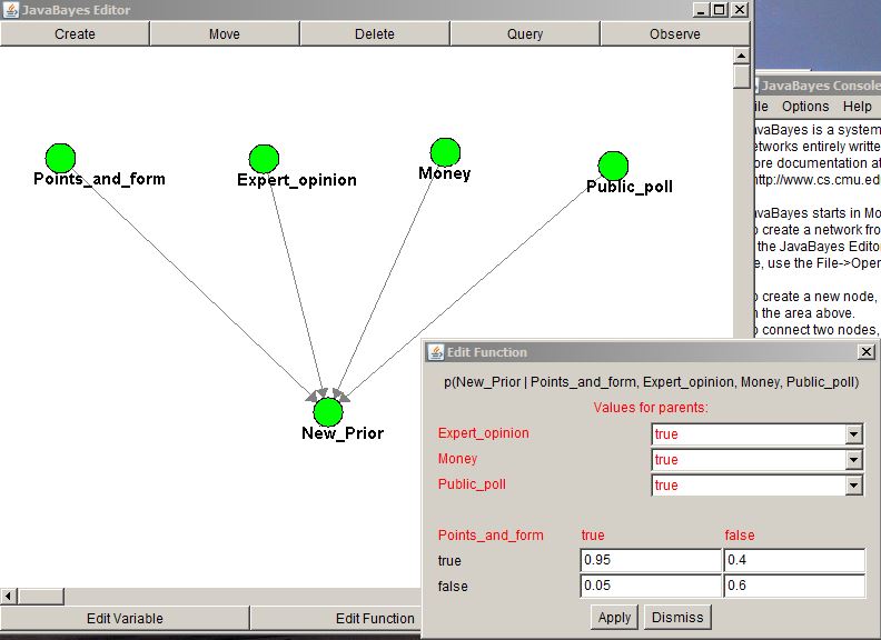
This was done by setting up a Bayesian belief network using JavaBayes (available here), in the same way as for the political data previously.  In this case, all four data sets fed into a final posterior distribution (however, as this was to be used in further analysis, it was called the ‘new prior’). The nice aspect of JavaBayes here is that it becomes intuitive that some parts of the data deserve more weighting than other parts. For example, in the screen shot below, it is clear that the previous form is given more weighting than the other variables (if form suggests the team will not make the top 4 – i.e. it is FALSE, but all the other variables suggest they will make the top 4, then there is only a 0.4 probability that they will in fact make the top four (in these calculations). Full details of the probabilities used are in the XML file (here – right click and ‘Save link as’ to access) which can be loaded into JavaBayes.

Importance of form

Interactions between teams:

From previous form and current (at the start of January) points, we identified 8 teams which could finish in the top 4. However, there are interactions between teams – if one wins, then by default, the one they play against loses. Equally there are only 4 places in the top 4 (an obvious fact, but perhaps one that needs stating…). So, if one team are in the top 4, then this means the chances of others getting there are decreased.

Incorporating reciprocal interactions in Bayesian networks is difficult statistically, and as such not really done in an intuitive manner by most BBN software. However, it is quite easy computationally (see here for details). This Excel file, with associated VBA code, runs reciprocal interactions – how it works can probably be followed from this paper.  In this case, the interaction probabilities (the third tab of the worksheet) are key. It is obvious from the data above that Man City and Chelsea will be extremely unlikely to finish outside the top 4. Hence, really the competition is for the remaining two places. Hence interaction strengths between teams and either Chelsea of Man City are weaker than for the others (closer to 0.5, meaning equal chance of being or not being in the top 4).

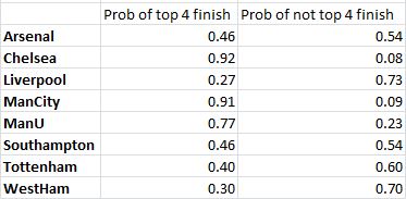
Running the simulation produces the following predictions:

FinalPredict


So, top 4 finishes likely for Chelsea, Man City and Man U. The final place is equally likely to be either Southampton or Arsenal (based on predictions and data from the start of 2015).

The current (24th Feb) positions are (and yes, this is my first look at this, since early Jan):

Table24thFeb

So, these really are looking pretty good at the moment.

Posted in Uncategorized | Comments Off on Champions’ League

Simple interactions – the rise of UKIP

In my previous post, I made the insinuation that election commentators had no idea who would win the election. Broadly this is true, but of course, when you are paid to write opinion, you have to say more than this. The biggest factor they talk about is UKIP. At the start of January, it was generally thought that UKIP would take most votes from the Conservatives, but would also still take some votes from labour. However, a rise in support for UKIP would favour Labour as the winning party, a decline in votes for UKIP would favour the conservatives.

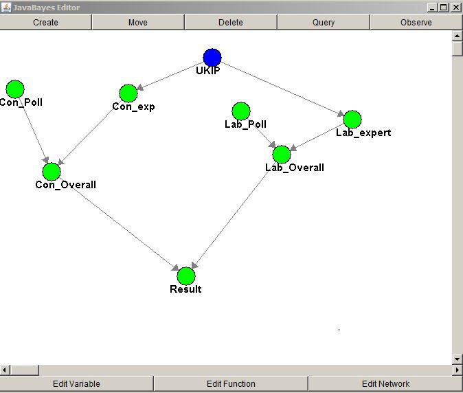
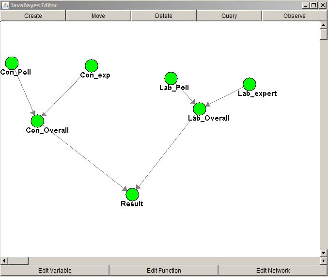
In this case, we have a simple interaction – UKIP influences labour and conservative (we don’t really need to consider the reciprocal, it’s unlikely UKIP will get the most votes, even if they get a lot). Bayesian belief networks handle these simple interactions well. We have a new structure for the network:

Network_advanced

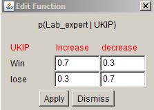
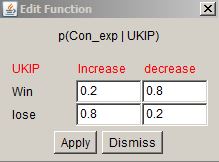
And some new functions – quite simple, what will happen to expert opinion should UKIP votes increase (or decrease). Everything else is the same.

function4 function3

In the network, the UKIP node is blue. The reason for that is that this can be ‘observed’. Being observed gives the node a probability of 1 (of increasing – OR of decreasing). Of course, we can’t be that certain, but we can use this to help predict what might happen, depending on what happens to UKIP.

Fundamentally, if we don’t know what happens to UKIP, then the pollsters have no idea who will win. We get the same probabilities as before (62% likely for a labour win). However, if the UKIP vote decreases (let’s assume the highly unlikely event of Nigel Farage saying something offensive in the next 4 and a half months….. ) then we observe that the UKIP vote goes down and… it’s now only 53% likely that Labour will get the most votes.

Simple Bayesian belief networks are fine for these simple interactions – but let’s go back to the football. Only four teams can qualify for Europe, so if one becomes more likely, this should effect the chances of the others. Simple Bayesian networks don’t cope well with this – but in what is likely to be the final part of these blogs, I’ll show how this can be overcome and we can incorporate interaction, data and opinion to make some final predictions.

Posted in Uncategorized | Comments Off on Simple interactions – the rise of UKIP

Elections again – Bayesian belief networks and combining data types

One method of how to combine different types of data – especially qualitative and quantitative, is to convert both types into belief about a given event. The previous blog posts have demonstrated how to do this using different types of quantitative data – essentially they involve working out an actual percentage of a given event occurring, given some data which doesn’t directly lend itself to doing this.

However, converting qualitative data into beliefs (or probabilities between 1 and 0 of an event occurring) is actually easier. Essentially it is just educated guess work. An easy example – expert opinion on who will win the most votes in the general election is largely – It is too close to call. A justification of that can be found in this paragraph from the Observer newspaper (see here for full article – http://www.theguardian.com/politics/2014/dec/27/2015-general-election-unpredictable-green-party-ukip:

“Political pundits are hedging their bets as never before. Their crystal balls reveal only a thick fog of uncertainty. They can agree on one thing – that it is impossible to say who will be prime minister after the election in five months’ time. “The 2015 election is the most unpredictable in living memory,” says Robert Ford, co-author of a book about the rise of Ukip, Revolt on the Right. “Past elections have been close but none has featured as many new and uncertain factors with the capacity to exert a decisive impact on the outcome.””

So, in answer to the question – will the Conservatives get the most votes – the belief is simple – 0.5, or I have no idea… there’s a 50:50 chance…

It’s easy enough to combine this (possibly not insightful, but at least honest) expert opinion with our predictions from yesterday’s opinion poll analysis using a Bayesian belief network (BBN). The following diagram (and parameterised belief network) was made in the free JavaBayes software, available here: http://www.cs.cmu.edu/~javabayes/Home/

You can download the code for the network (in XML format) here
http://www.rickstafford.com/software/basic_network.xml

Network

It’s not as scary as it all looks, essentially a BBN is just a way of formalising combining probabilities, although it does use the standard Bayesian equation to do so. However, the ‘Beliefs’ from yesterday’s opinion poll analysis are combined with the ‘expert’ opinion (the 50:50 split) to give an overall probability of each party winning the most votes. The final node then tells us the probability of Labour or the Conservatives having the most votes (in this case, they do add to one, as no other party is thought to be able to actually get the highest number of votes).

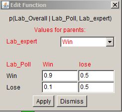
There are some simple functions to include here – for example, how do we weight the different types of evidence? The function is simple enough to complete, and looks like this:

Function

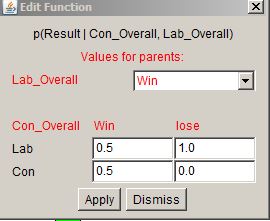
What it means is, given that the opinion poll data AND expert opinion both indicate labour is definitely winning (i.e. have values of 1) then the probability of labour winning in reality (given the election is a long time away) will be 90%. In practice, the input values (or priors, if you like) are not 1, but are 0.97 and 0.5 respectively. Combining these gives a probability of labour getting the most votes of 69%. Such an approach seems realistic – if expert opinion was absolutely certain that Labour would win, and they were even higher in the opinion polls, then even with 4 months to the election, it would seem right that we would be 90% sure of the final result. Incidentally, the odds of the Conservatives getting the most votes is 0.312 (essentially through the same parameter set) – at this point they add up to 1, but this isn’t essential at this point, as there is a final node to consider.

The final node in the BBN provides the result – the function for working this out looks like this:

Function2

Essentially, if the node has data from the two feeding nodes that Labour win (with probability 1) and Conservatives lose (with probability 0 of winning) then it calls a Labour win. If the two nodes disagree, then it doesn’t know what to make of it. The final node here gives the following outcome:
Labour 69%, Conservatives 31% – identical to before, but this is because both sides of the network are in agreement. If they weren’t, then we’d get a different result here.

As you can see, we’ve now combined two types of data to get a better prediction of the current state of knowledge (based on data on or before 4th Jan) as to who will win the election. Why is this a better prediction? Because the opinion poll alone is a snapshot in time, and very likely to change once campaign starts. The expert opinion recognises this and moderates the results.

Next I’ll look at how to combine semi-opinion, semi-quantitative data together. The election story becomes a bit more complicated, as experts haven’t stopped at the ‘I don’t know’ stage, but have taken a more in depth analysis – and obviously football pundits have a lot to say…

Posted in Uncategorized | Comments Off on Elections again – Bayesian belief networks and combining data types

Probability of winning an election

While the time to the UK general election is roughly the same as that to the end of the football season (see here), there are considerable differences in the type of data presented on which to make predictions. The biggest difference is that for the football league tables, half of the games have already been played – and those points are ‘in the bag’. For the election, nothing has been decided. However, a good place to start the predictions is with opinion polls. The opinion polls at the start of January (Guardian/ICM – 17th Dec) gave the following.

Conservatives – 28%
Labour – 33%
Lib Dem – 14%
UKIP – 14%
Green 5%
Others 6%

The question I want answered is: What is the likelihood of the conservatives getting the most number of votes at the election. This is a very different question from who will win the most seats, who the prime minister will be and so on. But again, as with the football league the conversion of the data above to answer the question I want to ask isn’t straightforward. Here’s how I approached it.

Typically, there is a margin of error of 3% in a typical opinion poll (based only on the sample size of people tested). The margin of error is calculated as follows:

1.96 * (√((p.q)/n))

The important bit here being the 1.96, indicating in fact it is 95% likely (given a normal distribution) that the real margin of error falls in the limit given. However, assuming the normal distribution (and in the absence of other information), this means we can simulate scenarios based the standard deviation of the error being 3/1.96.

So, to simulate the actual percentage of votes cast for any party, we calculate a random number from a normal distribution with the mean as the value above for each party, and the SD as 3/1.96.

If we replicate this a lot of times (10,000) then we can calculate what we are in fact interested in -the likelihood of the conservatives getting the most votes. This means their percentage of the vote must be higher than labour’s.

The simulation gives a probability of 2.73% for the conservatives getting the most votes, compared to labour’s 97.27. Given the percentage in the opinion polls, no other parties stand a chance.

However, the total number of votes must add to 100%, and the current simulation does not account for this. If we enforce this addition to 100% – basically each party’s percentage is out by a certain margin of error, and we will only count replicate runs where the total for all parties sums to 100, then we get a slightly different result – a 3.39% chance of getting the most votes, compared to 96.61 for Labour. The difference is still there on multiple runs of this simulation, probably because it is more likely that a margin of error in favour of the conservatives would be offset by a margin of error against Labour (more likely, not definite).

So, there we have it – values from the quantitative data which I can begin to use. There are a number of factors which need to be taken into account to give me the best possible prediction, and given that manifestos are not written yet, expert opinion may be very important here. How these get combined will be the subject of further posts.

R code for these simulations is given here.

Posted in Uncategorized | Comments Off on Probability of winning an election

Who will get to Europe?

The UK football season is just over halfway through its year. The top four teams will qualify for the European Champions league, and that means a lot of money. So, what is the probability that any given team will actually qualify? We have a league table, giving positions and points of each team, so we have some knowledge of the season so far, current form of the teams and so on. So how can I calculate the probability that a team will qualify? For my Bayesian belief network I want some prior values – probabilities between 0 and 1 that this may occur.

My solution is this:

I work out the overall form of the team this season (I am not considering current form, recent form, changes in management or anything else at the moment).

Prob of winning = Games Won / Games Played

And the same for drawing and losing

I then simulate all remaining games (18 for each team on the 4th Jan)

Suppose I take Chelsea, currently top of the table:

Won 14, drawn 4, lost 2

Prob of winning = 14/20 = 0.7
Prob of drawing = 4/20 = 0.2
Prob of losing = 2/20 = 0.1

So for each game, I generate a random number between 0 and 1. If it is less than 0.1, I assume they lose, if it is between 0.1 and 0.3, they draw, if it is over 0.3, they win.

I do this for all 20 teams, then calculate their points (3 for each win, 1 for each draw). I then pick the highest four teams. As I am only interested in the top four teams, I am not worried if aspects of these calculations are not fully correct – for example, in this calculation, all the top teams could (although it is unlikely) win all their remaining games. In practice, this could not happen, as they will have to play each other and they can’t all win these games.

Since this is all highly stochastic, I run the simulation 10,000 times and calculate the percentage of times each team ends up in the top four – this gives me my probability.

So, for those of you interested, here are the probabilities – if your team isn’t here, then they have no chance, sorry….

Arsenal – 20.01%
Chelsea – 99.99%
Liverpool – 2.19%
Man City – 99.99%
Man United – 71.53%
Newcastle – 0.32%
Southampton – 59.54%
Stoke City – 0.19%
Swansea City – 2.12%
Tottenham – 31.12%
West Ham – 13.00%

The R code for the calculations may be horribly inefficient, but is available here (it took an hour to calculate, so if you want to play with it, then reduce the bootstrap size).

The league table as of the 4th Jan – formatted for the R code – is here.

Of course, there should be consideration of new players, current form, new managers and so on, and that is something which can be built on, now I have my probabilities. More to come on this in the next few days

Posted in Uncategorized | 1 Comment